 Dynamic programming.
Did you feel a little shiver when you read that?
Imagine it again with those spooky Goosebumps letters.
Dynamic programming.
When I talk to students of mine over at Byte by Byte, nothing quite strikes fear into their hearts like dynamic programming.
And I can totally understand why. Dynamic programming (DP) is as hard as it is counterintuitive. Most of us learn by looking for patterns among different problems. But with dynamic programming, it can be really hard to actually find the similarities.
Even though the problems all use the same technique, they look completely different.
However, there is a way to understand dynamic programming problems and solve them with ease. And in this post I’m going to show you how to do just that.
What Is Dynamic Programming?
Before we get into all the details of how to solve dynamic programming problems, it’s key that we answer the most fundamental question:
What is dynamic programming?
Simply put, dynamic programming is an optimization technique that we can use to solve problems where the same work is being repeated over and over. You know how a web server may use caching? Dynamic programming is basically that.
However, dynamic programming doesn’t work for every problem. There are a lot of cases in which dynamic programming simply won’t help us improve the runtime of a problem at all. If we aren’t doing repeated work, then no amount of caching will make any difference.
To determine whether we can optimize a problem using dynamic programming, we can look at both formal criteria of DP problems. I’ll also give you a shortcut in a second that will make these problems much quicker to identify.
Let’s start with the formal definition.
A problem can be optimized using dynamic programming if it:
- has an optimal substructure.
- has overlapping subproblems.
If a problem meets those two criteria, then we know for a fact that it can be optimized using dynamic programming.
Optimal Substructure
Optimal substructure is a core property not just of dynamic programming problems but also of recursion in general. If a problem can be solved recursively, chances are it has an optimal substructure.
Optimal substructure simply means that you can find the optimal solution to a problem by considering the optimal solution to its subproblems.
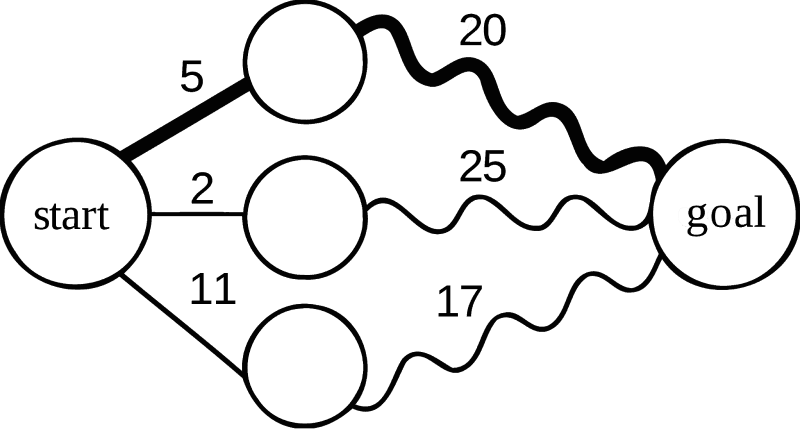
For example, if we are looking for the shortest path in a graph, knowing the partial path to the end (the bold squiggly line in the image below), we can compute the shortest path from the start to the end, without knowing any details about the squiggly path.
What might be an example of a problem without optimal substructure?
Consider finding the cheapest flight between two airports. According to Wikipedia:
“Using online flight search, we will frequently find that the cheapest flight from airport A to airport B involves a single connection through airport C, but the cheapest flight from airport A to airport C involves a connection through some other airport D.”
While there is some nuance here, we can generally assume that any problem that we solve recursively will have an optimal substructure.
Overlapping Subproblems
Overlapping subproblems is the second key property that our problem must have to allow us to optimize using dynamic programming. Simply put, having overlapping subproblems means we are computing the same problem more than once.
Imagine you have a server that caches images. If the same image gets requested over and over again, you’ll save a ton of time. However, if no one ever requests the same image more than once, what was the benefit of caching them?
This is exactly what happens here. If we don’t have overlapping subproblems, there is nothing to stop us from caching values. It just won’t actually improve our runtime at all. All it will do is create more work for us.
For an example of overlapping subproblems, consider the Fibonacci problem. Here is a tree of all the recursive calls required to compute the fifth Fibonacci number:
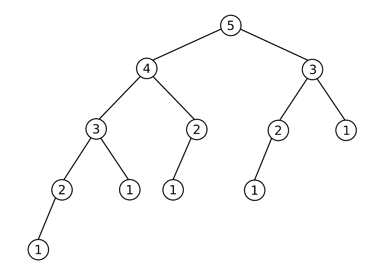
Notice how we see repeated values in the tree. The number 3 is repeated twice, 2 is repeated three times, and 1 is repeated five times. Each of those repeats is an overlapping subproblem. There is no need for us to compute those subproblems multiple times because the value won’t change. If we cache it, we can save ourselves a lot of work.
When Should I Use Dynamic Programming?
To be absolutely certain that we can solve a problem using dynamic programming, it is critical that we test for optimal substructure and overlapping subproblems. Without those, we can’t use dynamic programming.
However, we can use heuristics to guess pretty accurately whether or not we should even consider using DP. This quick question can save us a ton of time.
All we have to ask is: Can this problem be solved by solving a combination problem?
Consider a few examples:
- Find the smallest number of coins required to make a specific amount of change. Look at all combinations of coins that add up to an amount, and count the fewest number.
- Find the most value of items that can fit in your knapsack. Find all combinations of items and determine the highest value combination.
- Find the number of different paths to the top of a staircase. Enumerate all the combinations of steps.
While this heuristic doesn’t account for all dynamic programming problems, it does give you a quick way to gut-check a problem and decide whether you want to go deeper.
Solve Any DP Problem Using the FAST Method
After seeing many of my students from Byte by Byte struggling so much with dynamic programming, I realized we had to do something. There had to be a system for these students to follow that would help them solve these problems consistently and without stress.
It was this mission that gave rise to The FAST Method.
The FAST Method is a technique that has been pioneered and tested over the last several years. As I write this, more than 8,000 of our students have downloaded our free e-book and learned to master dynamic programming using The FAST Method.
So how does it work?
FAST is an acronym that stands for Find the first solution, Analyze the solution, identify the Subproblems, and Turn around the solution. Let’s break down each of these steps.
Find the First Solution
The first step to solving any dynamic programming problem using The FAST Method is to find the initial brute force recursive solution.
Your goal with Step One is to solve the problem without concern for efficiency. We just want to get a solution down on the whiteboard. This gives us a starting point (I’ve discussed this in much more detail here).
There are a couple of restrictions on how this brute force solution should look:
- Each recursive call must be self-contained. If you are storing your result by updating some global variable, then it will be impossible for us to use any sort of caching effectively. We want to have a result that is completely dependent on the inputs of the function and not affected by any outside factors.
- Remove unnecessary variables. The fewer variables you pass into your recursive function, the better. We will be saving our cached values based on the inputs to the function, so it will be a pain if we have extraneous variables.
Let’s consider two examples here. We’ll use these examples to demonstrate each step along the way.
Example 1:
The first problem we’re going to look at is the Fibonacci problem. In this problem, we want to simply identify the n-th Fibonacci number. Recursively we can do that as follows:
// Compute the nth Fibonacci number
// We assume that n >= 0 and that int is sufficient to hold the result
int fib(int n) {
if (n == 0) return 0;
if (n == 1) return 1;
return fib(n-1) + fib(n-2);
}
It is important to notice here how each result of fib(n) is 100 percent dependent on the value of “n.” We have to be careful to write our function in this way. For example, while the following code works, it would NOT allow us to do DP.
// Compute the nth Fibonacci number
// We assume that n >= 0 and that int is sufficient to hold the result
int fib(int n) {
int result = 0;
fibInner(n, &result);
return result;
}
void fibInner(int n, int *result) {
*result += n;
if (n == 0 || n == 1) return;
fibInner(n-1, result);
fibInner(n-2, result);
}
While this may seem like a toy example, it is really important to understand the difference here. This second version of the function is reliant on result to compute the result of the function and result is scoped outside of the fibInner() function.
You can learn more about the difference here.
Example 2:
The second problem that we’ll look at is one of the most popular dynamic programming problems: 0-1 Knapsack Problem. For this problem, we are given a list of items that have weights and values, as well as a max allowable weight. We want to determine the maximum value that we can get without exceeding the maximum weight.
Here is our brute force recursive code:
public class Item { int weight; int value; } class Item { int weight; int value; } // Brute force solution int bruteForceKnapsack(Item[] items, int W) { return bruteForceKnapsack(items, W, 0); } // Overloaded recursive function int bruteForceKnapsack(Item[] items, int W, int i) { // If we've gone through all the items, return if (i == items.length) return 0; // If the item is too big to fill the remaining space, skip it if (W - items[i].weight < 0) return bruteForceKnapsack(items, W, i+1);// Find the maximum of including and not including the current item return Math.max(bruteForceKnapsack(items, W - items[i].weight, i+1) + items[i].value, bruteForceKnapsack(items, W, i+1)); }
With these brute force solutions, we can move on to the next step of The FAST Method.
Note: I’ve found that many people find this step difficult. It is way too large a topic to cover here, so if you struggle with recursion, I recommend checking out this monster post on Byte by Byte.
Analyze the First Solution
Now that we have our brute force solution, the next step in The FAST Method is to analyze the solution. In this step, we are looking at the runtime of our solution to see if it is worth trying to use dynamic programming and then considering whether we can use it for this problem at all.
We will start with a look at the time and space complexity of our problem and then jump right into an analysis of whether we have optimal substructure and overlapping subproblems. Remember that those are required for us to be able to use dynamic programming.
Let’s go back to our Fibonacci example.
Example 1 (Fibonacci):
For this problem, our code was nice and simple, but unfortunately our time complexity sucks. The easiest way to get a handle on what is going on in your code is to sketch out the recursive tree. Here’s the tree for fib(4):
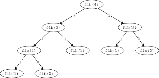
What we immediately notice here is that we essentially get a tree of height n. Yes, some of the branches are a bit shorter, but our Big Oh complexity is an upper bound. Therefore, to compute the time complexity, we can simply estimate the number of nodes in the tree.
For any tree, we can estimate the number of nodes as branching_factorheight, where the branching factor is the maximum number of children that any node in the tree has. That gives us a pretty terrible runtime of O(2n).
So it would be nice if we could optimize this code, and if we have optimal substructure and overlapping subproblems, we could do just that.
In this case, we have a recursive solution that pretty much guarantees that we have an optimal substructure. We are literally solving the problem by solving some of its subproblems.
We also can see clearly from the tree diagram that we have overlapping subproblems. Notice fib(2) getting called two separate times? That’s an overlapping subproblem. If we drew a bigger tree, we would find even more overlapping subproblems.
Given that we have found this solution to have an exponential runtime and it meets the requirements for dynamic programming, this problem is clearly a prime candidate for us to optimize.
Example 2 (0-1 Knapsack):
The code for this problem was a little bit more complicated, so drawing it out becomes even more important. When we sketch out an example, it gives us much more clarity on what is happening (see my process for sketching out solutions).
Here’s what our tree might look like for the following inputs:
Items = {(w:2, v:6), (w:2, v:10), (w:3, v:12)}

maxWeight = 5
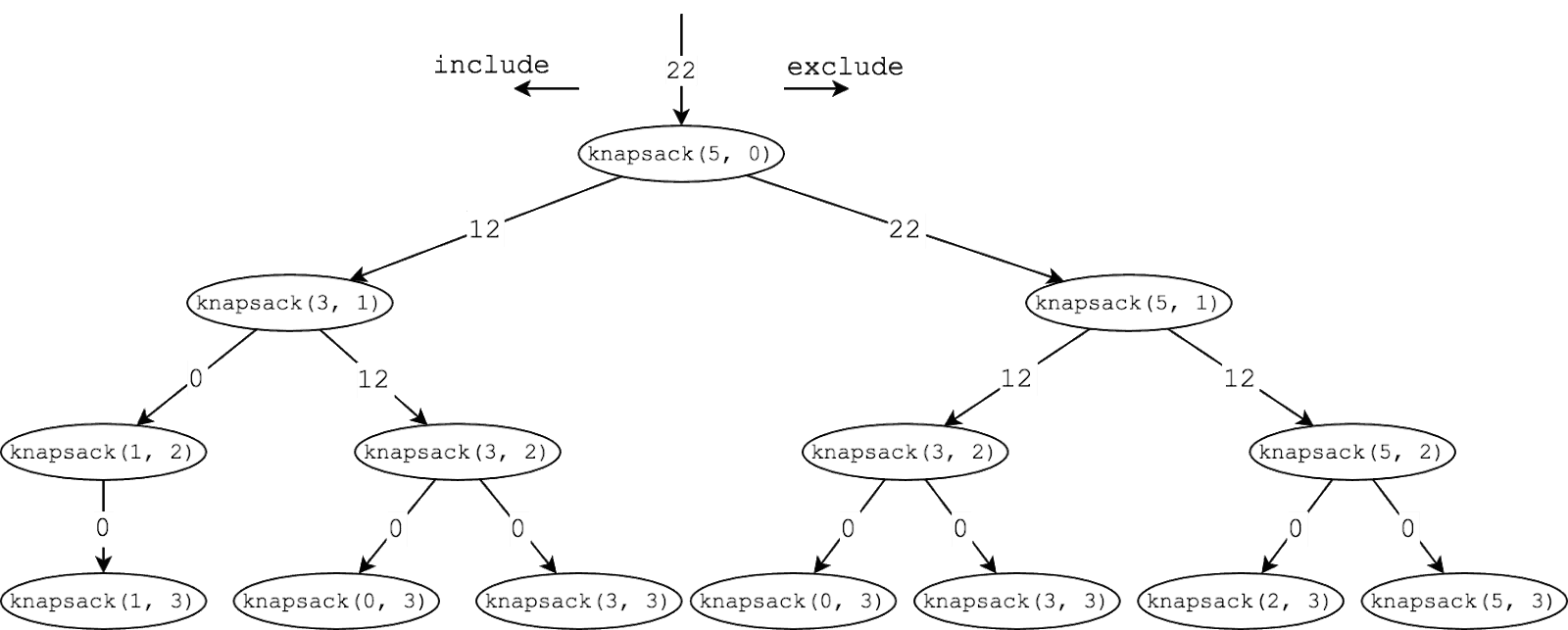
Note the two values passed into the function in this diagram are the maxWeight and the current index in our items list.
So with our tree sketched out, let’s start with the time complexity. Similar to our Fibonacci problem, we see that we have a branching tree of recursive calls where our branching factor is 2. This gives us a time complexity of O(2n).
Do we have optimal substructure? Yep. Again, the recursion basically tells us all we need to know on that count.
And overlapping subproblems? Since we’ve sketched it out, we can see that knapsack(3, 2) is getting called twice, which is a clearly overlapping subproblem.
This also looks like a good candidate for DP.
Identify the Subproblems
The third step of The FAST Method is to identify the subproblems that we are solving. This is where we really get into the meat of optimizing our code.
We are going to start by defining in plain English what exactly our subproblem is. I’m always shocked at how many people can write the recursive code but don’t really understand what their code is doing. Understanding is critical.
Once we understand the subproblems, we can implement a cache that will memoize the results of our subproblems, giving us a top-down dynamic programming solution.
Memoization is simply the strategy of caching the results. We can use an array or map to save the values that we’ve already computed to easily look them up later.
We call this a top-down dynamic programming solution because we are solving it recursively. Essentially we are starting at the “top” and recursively breaking the problem into smaller and smaller chunks. This is in contrast to bottom-up, or tabular, dynamic programming, which we will see in the last step of The FAST Method.
Example 1 (Fibonacci):
So what is our subproblem here? This problem is quite easy to understand because fib(n) is simply the nth Fibonacci number. Since our result is only dependent on a single variable, n, it is easy for us to memoize based on that single variable.
Consider the code below. By adding a simple array, we can memoize our results. Notice the differences between this code and our code above:
// Top-down dynamic solution
int topDownFib(int n) {
int[] dp = new int[n+1];
return topDownFib(n, dp);
}
// Overloaded private method
int topDownFib(int n, int[] dp) {
if (n == 0 || n == 1) return n;
// If value is not set in cache, compute it
if (dp[n] == 0) {
dp[n] = topDownFib(n-1, dp) + topDownFib(n-2, dp);
}
return dp[n];
}
See how little we actually need to change? Once we understand our subproblem, we know exactly what value we need to cache.
Now that we have our top-down solution, we do also want to look at the complexity. In this case, our code has been reduced to O(n) time complexity. We can pretty easily see this because each value in our dp array is computed once and referenced some constant number of times after that. This is much better than our previous exponential solution.
Example 2 (0-1 Knapsack):
This problem starts to demonstrate the power of truly understanding the subproblems that we are solving. Specifically, not only does knapsack() take in a weight, it also takes in an index as an argument. So if you call knapsack(4, 2) what does that actually mean? What is the result that we expect? Well, if you look at the code, we can formulate a plain English definition of the function:
Here, “knapsack(maxWeight, index) returns the maximum value that we can generate under a current weight only considering the items from index to the end of the list of items.”
With this definition, it makes it easy for us to rewrite our function to cache the results (and in the next section, these definitions will become invaluable):
// Top-down dynamic solution
int topDownKnapsackArray(Item[] items, int W) {
int[][] dp = new int[items.length][W + 1];
for (int i = 0; i < dp.length; i++) {
for (int j = 0; j < dp[0].length; j++) {
dp[i][j] = -1;
}
}
return topDownKnapsackArray(items, W, 0, dp);
}
// Overloaded recursive function
int topDownKnapsackArray(Item[] items, int W, int i, int[][] dp) {
if (i == items.length) return 0;
if (dp[i][W] == -1) {
dp[i][W] = topDownKnapsackArray(items, W, i+1, dp);
if (W - items[i].weight >= 0) {
int include = topDownKnapsackArray(items, W-items[i].weight, i+1, dp) + items[i].value;
dp[i][W] = Math.max(dp[i][W], include);
}
}
return dp[i][W];

}
Again, we can see that very little change to our original code is required. All we are doing is adding a cache that we check before computing any function. If the value in the cache has been set, then we can return that value without recomputing it.
In terms of the time complexity here, we can turn to the size of our cache. Each value in the cache gets computed at most once, giving us a complexity of O(n*W).
Turn Around the Solution
The final step of The FAST Method is to take our top-down solution and “turn it around” into a bottom-up solution. This is an optional step, since the top-down and bottom-up solutions will be equivalent in terms of their complexity. However, many prefer bottom-up due to the fact that iterative code tends to run faster than recursive code.
With this step, we are essentially going to invert our top-down solution. Instead of starting with the goal and breaking it down into smaller subproblems, we will start with the smallest version of the subproblem and then build up larger and larger subproblems until we reach our target. This is where the definition from the previous step will come in handy.
Example 1 (Fibonacci):
To start, let’s recall our subproblem: fib(n) is the nth Fibonacci number.
Remember that we’re going to want to compute the smallest version of our subproblem first. That would be our base cases, or in this case, n = 0 and n = 1.
Once we have that, we can compute the next biggest subproblem. To get fib(2), we just look at the subproblems we’ve already computed. Once that’s computed we can compute fib(3) and so on.
So how do we write the code for this? Well, our cache is going to look identical to how it did in the previous step; we’re just going to fill it in from the smallest subproblems to the largest, which we can do iteratively.
// Bottom-up dynamic solution
int bottomUpFib(int n) {
if (n == 0) return 0;
// Initialize cache
int[] dp = new int[n+1];
dp[1] = 1;

// Fill cache iteratively
for (int i = 2; i <= n; i++) {
dp[i] = dp[i-1] + dp[i-2];
}


return dp[n];

}
Easy peasy lemon squeezy.
Another nice perk of this bottom-up solution is that it is super easy to compute the time complexity. Unlike recursion, with basic iterative code it’s easy to see what’s going on.
And that’s all there is to it. One note with this problem (and some other DP problems) is that we can further optimize the space complexity, but that is outside the scope of this post.
Example 2 (0-1 Knapsack):
As is becoming a bit of a trend, this problem is much more difficult. However, you now have all the tools you need to solve the Knapsack problem bottom-up.
Recall our subproblem definition: “knapsack(maxWeight, index) returns the maximum value that we can generate under a current weight only considering the items from index to the end of the list of items.”
To make things a little easier for our bottom-up purposes, we can invert the definition so that rather than looking from the index to the end of the array, our subproblem can solve for the array up to, but not including, the index.
With this, we can start to fill in our base cases. We’ll start by initializing our dp array. Whenever the max weight is 0, knapsack(0, index) has to be 0. Referring back to our subproblem definition, that makes sense. If the weight is 0, then we can’t include any items, and so the value must be 0.
The same holds if index is 0. Since we define our subproblem as the value for all items up to, but not including, the index, if index is 0 we are also including 0 items, which has 0 value.
From there, we can iteratively compute larger subproblems, ultimately reaching our target:
// Bottom-up dynamic solution.
int bottomUpKnapsack(Item[] items, int W) {
if (items.length == 0 || W == 0) return 0;
// Initialize cache
int[][] dp = new int[items.length + 1][W + 1];
// For each item and weight, compute the max value of the items up to
// that item that doesn't go over W weight
for (int i = 1; i < dp.length; i++) {
for (int j = 0; j < dp[0].length; j++) {
if (items[i-1].weight > j) {
dp[i][j] = dp[i-1][j];
} else {
int include = dp[i-1][j-items[i-1].weight] + items[i-1].value;
dp[i][j] = Math.max(dp[i-1][j], include);
}

}

}

return dp[items.length][W];

}
Again, once we solve our solution bottom-up, the time complexity becomes very easy because we have a simple nested for loop.
Dynamic Programming Doesn’t Have to Be Hard!
While dynamic programming seems like a scary and counterintuitive topic, it doesn’t have to be. By applying structure to your solutions, such as with The FAST Method, it is possible to solve any of these problems in a systematic way.
Interviewers love to test candidates on dynamic programming because it is perceived as such a difficult topic, but there is no need to be nervous. Follow the steps and you’ll do great.
If you want to learn more about The FAST Method, check out my free e-book, Dynamic Programming for Interviews.

Related Articles

12 REALITIES of Daily Life as a Programmer
What’s the daily life of a programmer like? A programmer’s daily life consists of auditing and debugging code, coding new…

5G App Development: How To Prepare for the Future of the Internet
5G is the fifth generation of broadband cellular mobile networks and is expected to bring a huge change in the…
Impostor Syndrome as a Programmer
Believing that you’re somewhat unqualified for your job is a problem faced by the best of us. When those thoughts…