
Data Science is a huge field. While there are many different focuses and skills available to learn, you don’t have to know all of them to consider yourself a data scientist. However, there is one thing you can’t do without: data—and the knowhow to manipulate it into a useful format.
Now, I’m not talking about “cleaning” data. That’s a huge topic in and of itself, and I could write a whole different article on it. I’m talking about after the data is clean, getting it into a representation that your analysis can understand, and even more powerfully, a representation that allows you to leverage the powerful, numerical analysis libraries that are available for fast, efficient, and clean analysis code.
While working on your data, you’ll frequently need to apply the same calculation to every single element of your data in order to get new data that’s the same shape. Let’s imagine that you have a million rows of data. Imagine writing a for-loop that loops through and visits each element. Ugh. Now imagine doing that for each step in your data analysis process. Now, you’ve got two data sets, and you want to compare each element in one to each element in the other, and you have to write a doubly nested for-loop for each calculation. Can you feel your code bloating? Can you feel your performance lagging? Can you feel your soul dying a little?
It is for these reasons (maybe not that last one) that the concepts of vectorization and broadcasting exist.
We’ll use powerful, vetted libraries written to capitalize on fast, compiled, low-level languages to do the heavy lifting for us. We’ll write the code that we want to write—that the mathematician inside each one of us wishes we could write.We’ll break the chains of the plain ’ole for-loop and discover the power of shaping our data. Because just like anything else, a little preparation goes a long way.
A woodsman was once asked, “What would you do if you had just five minutes to chop down a tree?” He answered, “I would spend the first two and a half minutes sharpening my ax.”
This article will have some examples that use Python and the NumPy package (which provides basic support for efficient vector operations). It should be clear enough for you to understand the ideas in this article even if you’re not a fluent Python user.
Vectorization
First, let’s talk about vectorization. To do that, we need to define what a vector is. A vector is nothing more than a collection of items that are all the same type—typically only in one dimension. A collection in two dimensions is often called a matrix. When talking about a generic collection with any number of dimensions, you can use the word array.
Note: The vocabulary will vary a little from language to language but will always mean “some collection of values.”
In data science cases, vectors are most often numbers, but other data types are possible as well. The idea behind vectorization is that if you’re careful, you can intuitively treat vectors just like single numbers.
Here is how vector math works:
In the same way you add two numbers together, you can add two vectors together, and the operation will be performed on an element-wise basis.
We have now “vectorized” the addition operation, making it work for vectors. The NumPy library has a whole bunch of vectorized functions, including square root, absolute value, trigonometry functions, logarithmic functions, exponential functions, and more.
These vectorized operations help take a lot of the mental load out of working with big collections of values when you basically want to do the same thing to all of them, treating the logic like you’re just working with one number. You don’t write any loops of your own!
Broadcasting
OK, so far we’ve figured out that the idea behind vectorization is to make operations between two collections of the same size and shape as intuitive as operations between two single numbers.
But what about when the collections are different shapes?
This is when we apply a concept known as broadcasting. Broadcasting is the act of extending an array to a shape that will allow it to successfully take part in a vectorized calculation. Here are the rules:
- If the two arrays are the same length in a dimension, that dimension will be operated on in an element-wise manner.
- If one array has some number in a dimension and the other array is only size 1 in that dimension, that value will be broadcast, and it will be used with each item in the other array.
- If the two arrays are different sizes and neither is size 1, broadcasting can’t be performed, and an error is thrown.
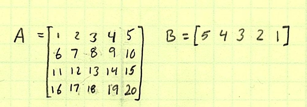
It’s a tough concept, so I think it’s time for some examples. First, let’s say we have one array that is 4×5 (four rows and five columns) and another one that is one row of five columns.
We have two dimensions to consider. In Axis 0 (the row axis), one is length 4, and the other is length 1. The rules are satisfied for broadcasting, so we broadcast!
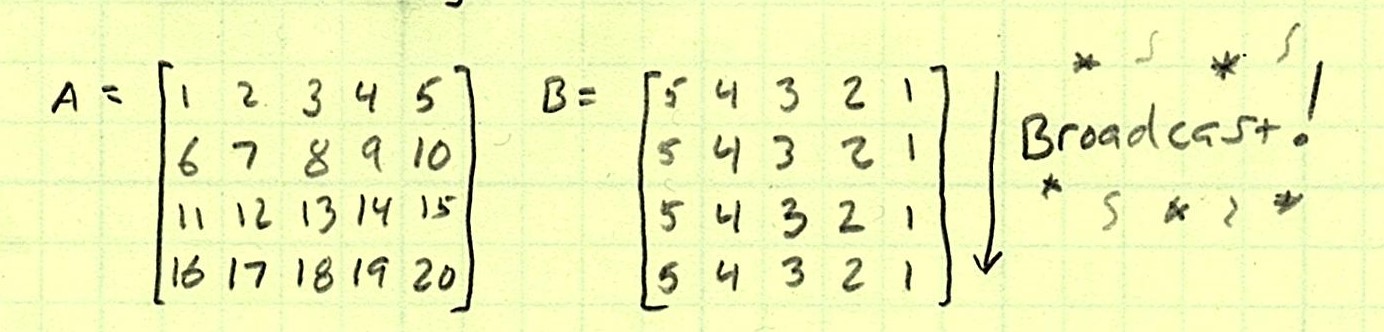
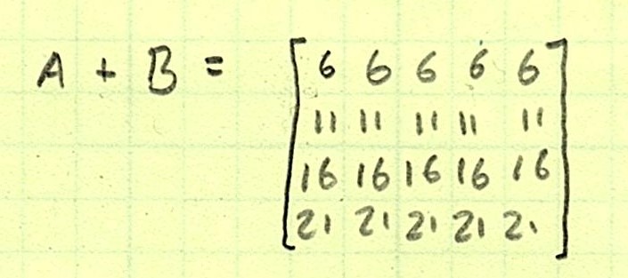
Now, Axis 0 matches. Checking Axis 1 (the column axis), both have five elements. Since they match, we can perform the operation.
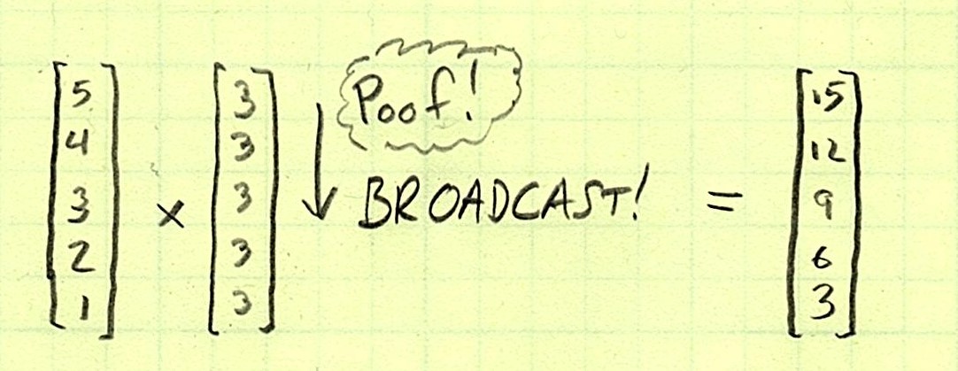
Let’s look at another example that is actually simpler but seems tricky at first:
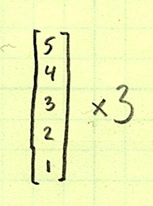
Just a regular number? Yes! You can think about this like a tiny 1x1x1 … array. It will be broadcast in as many axes as needed. In this case, we only need one.
OK. We’ve covered a little bit of what these concepts mean, how they work, and what they entail. But now it’s time to look at how we can use them and why we would even need to know about them. We’re going to go through an example that shows just how clean and fast they can make our data analysis code. By doing just a little bit of data-shaping setup, we can set ourselves up to knock the analysis out of the park with one simple, sweet line of logic.
The Orchid Dataset
Imagine we have a dataset on Orchids. This dataset is going to be split into two parts: a training set and a testing set. Using a “Nearest Neighbor” algorithm, we’re going to classify what kind of Orchids these are.
Now, what does all this mean?
Each row of the training set comes with four columns of floating point values describing different features of that particular plant: its lengths, widths, etc. Each row also comes with a label that says what species of Orchid it is.
Each row of the testing set has the same thing, but we’re going to compare each row in the testing set to the training set to try to predict what kind of Orchid it is.
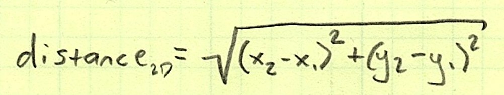
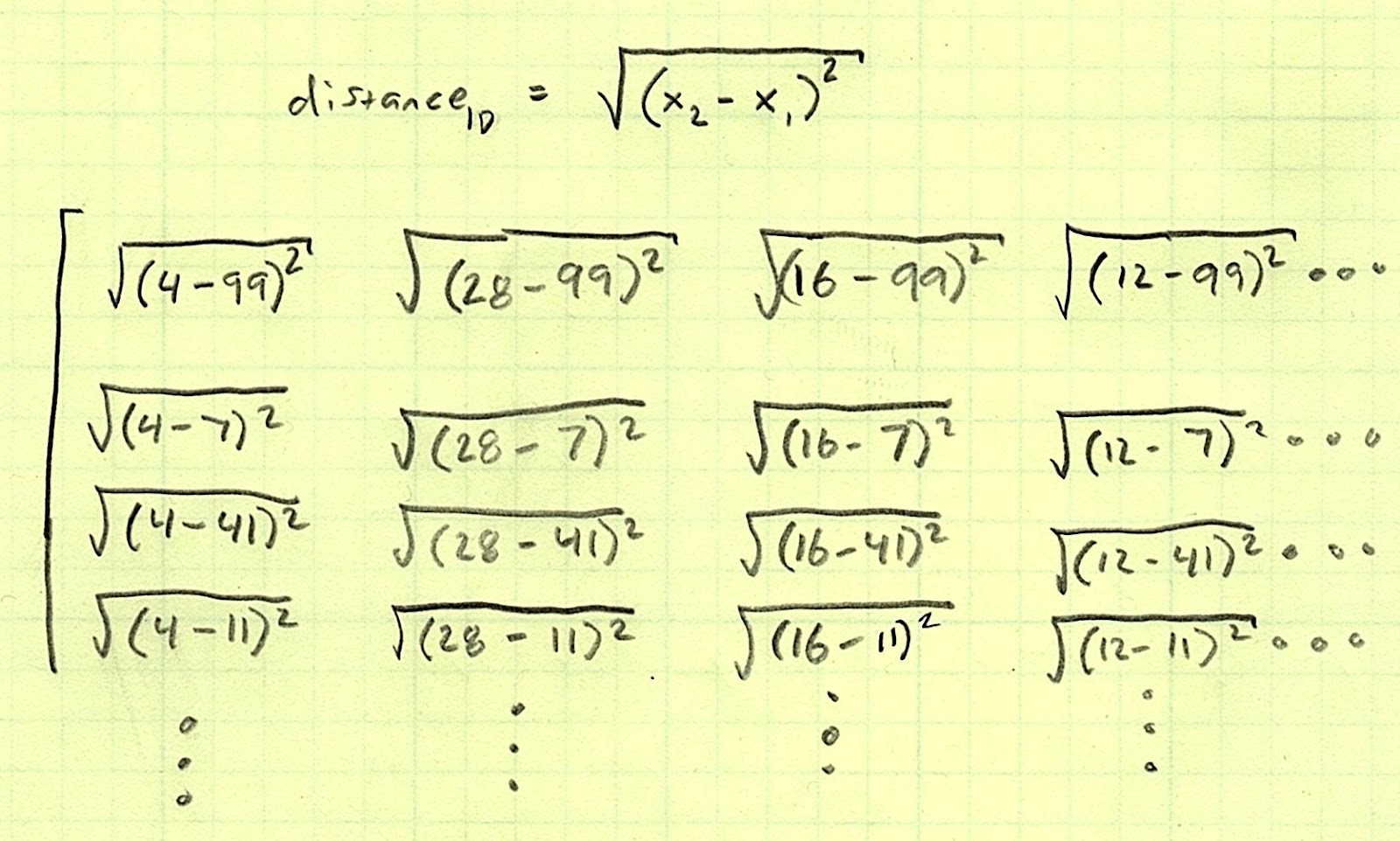
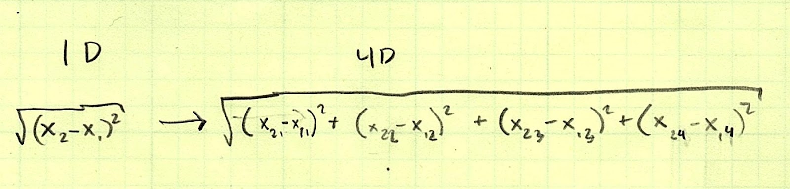
The “Nearest Neighbor” algorithm sounds a lot fancier than it is. We’re going to find out which row of the training set is “closest” to the row in the test set we’re trying to classify. By “closest,” I literally mean we are going to use a distance calculation. In 2D coordinates, you can calculate the distance between two points like this:
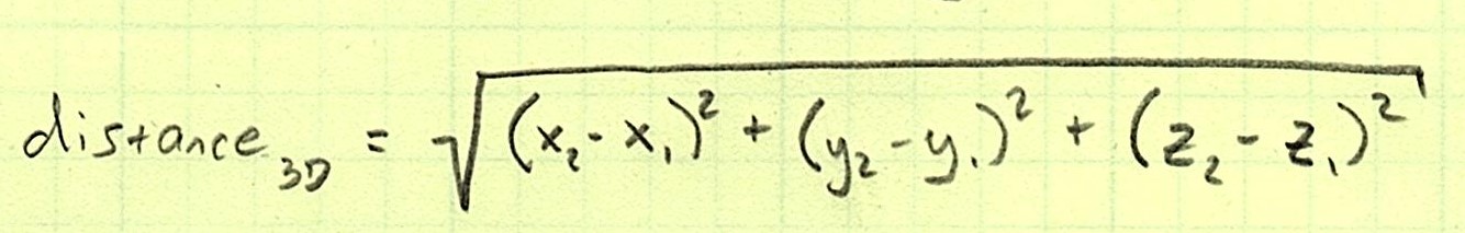
It doesn’t change much for 3D space:
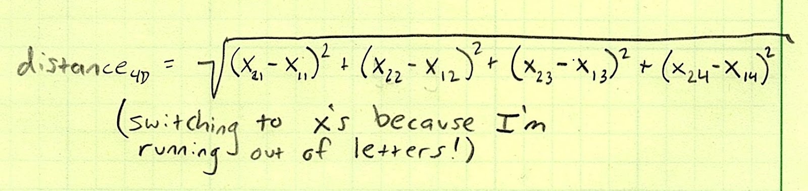
In fact, the pattern holds for any number of dimensions. We just so happen to have four:
So our goal is, for each row in the testing set, to:
- Find out which row in the training set is the most similar.
- Return the label of that “Nearest Neighbor” as our prediction for the label of that row in the testing set. (This makes sense because Orchids of the same species should mostly have very similar characteristics and be different from other species.)
But here’s how we’re going to stretch our array muscles: We’re going to do this without writing a single loop!
Before we see any code, we want to look at how we might achieve this in a simpler case because the fact that each orchid has four columns of data associated with it makes things just a tad bit harder.
A Simpler Case
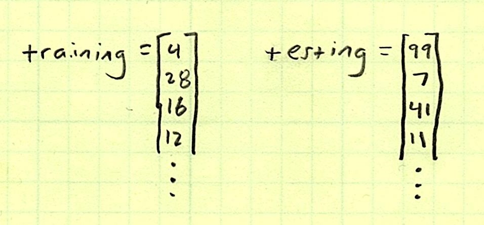
Let’s imagine we have an array of training numbers and an array of testing numbers.
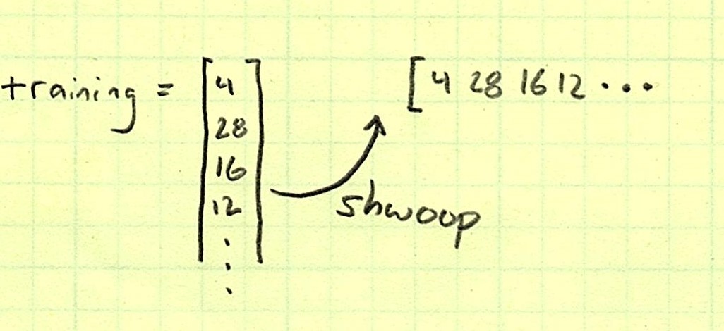
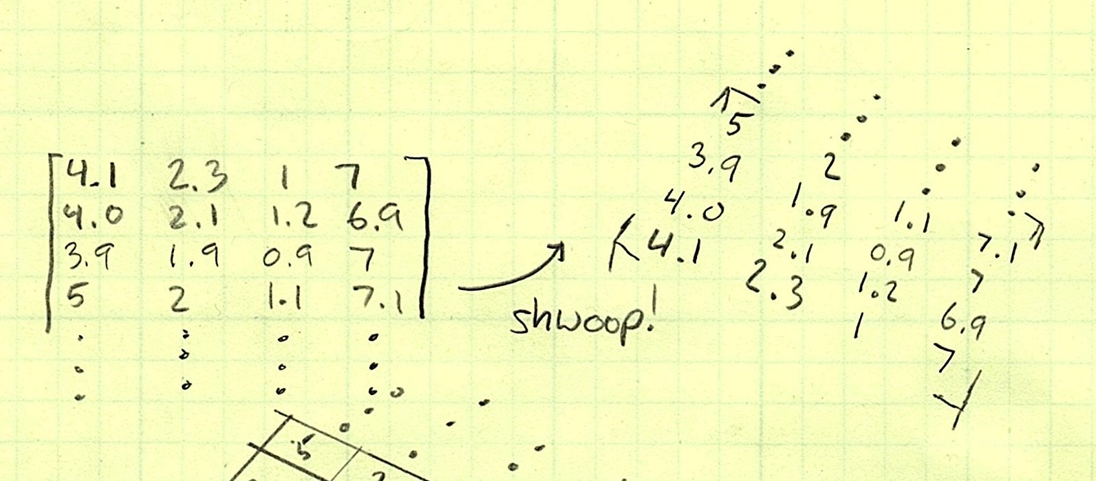
How can we use broadcasting to check each testing number against all training numbers? The trick is to rotate.
Remember that broadcasting only happens when you have length 1 in an axis where the other array has length more-than-one. So first we’ll convert training to a 2D array so it knows about the second dimension, and then we’ll swap axes so that instead of a single column, it is a single row—effectively rotating it up into a new dimension.
Now, training is 1×50, and testing is 50×1, so both arrays will be broadcasting in opposite dimensions!
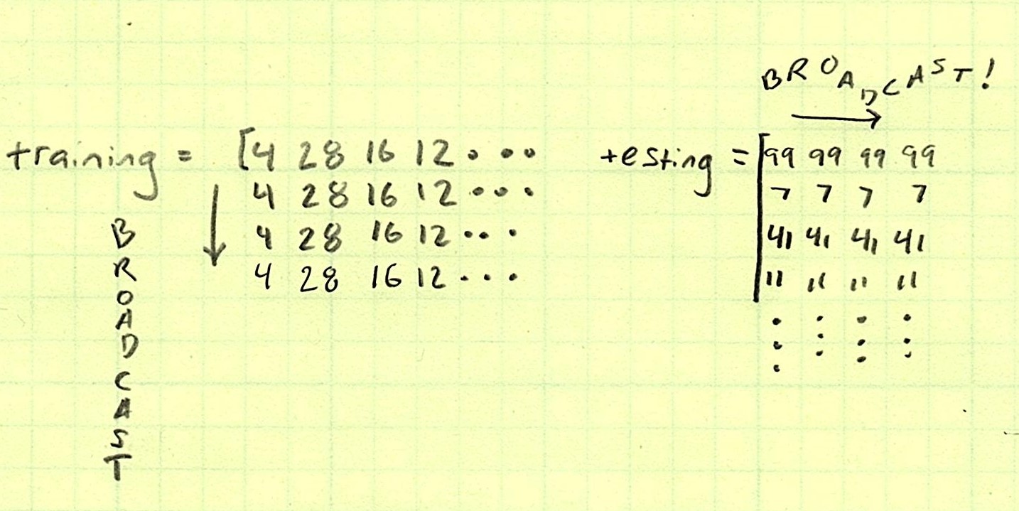
Through the amazing power of broadcasting, we’ve turned what was once a doubly nested loop into a single command that can now be used to do an element-wise distance calculation.
Back to the Orchids
OK, now that we’ve added the power of rotating arrays into new dimensions to our list of superpowers, let’s get back to our Orchids and see if we can apply the same techniques. The only difference is that our Orchids have four columns of data—an extra dimension! So what can we do? We’ve got a 75 x 4 testing set and a 75 x 4 training set. We can’t swap axes 0 and 1 because with 75 x 4 and 4 x 75, there’s no broadcasting. Remember the rules of broadcasting? We either need an axis with length 1, or we need the axes to be the same length. Can you see what we’re going to have to do?
We’re going into the …

That’s right. We can treat axis 1 (the four columns) like it’s something that doesn’t even bother us and rotate in a perpendicular direction instead!
Now we’ve got a 1 x 4 x 75 and a 75 x 4, so we’re almost there, but when we try to do any vectorized operations on them:
ValueError: operands could not be broadcast together with shapes (1,4,75) (75,4)
The testing dataset needs to at least acknowledge the existence of the third axis even if it doesn’t use it for anything.
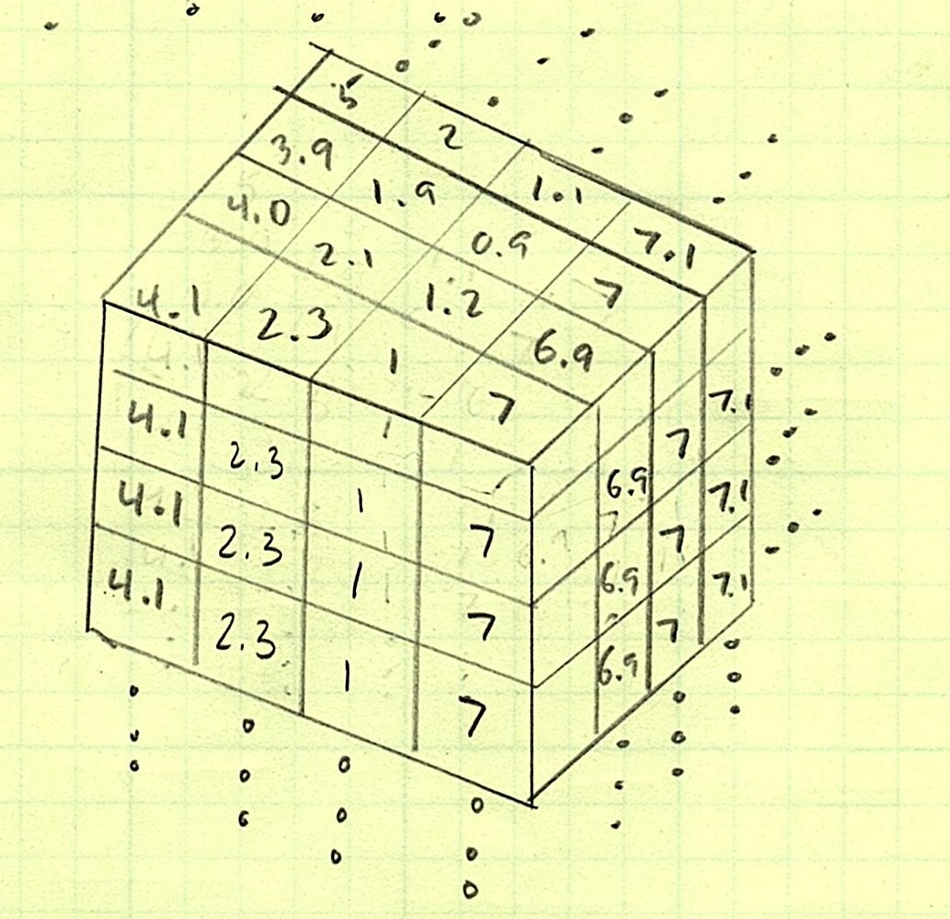
Finally, we’re here. We’ve got a 1 x 4 x 75 array and a 75 x 4 x 1 array. Same number of axes. Each axis either matches, or one of them is a 1, so we can broadcast. We’re ready. When we broadcast, it will look like this:
So how do we handle distance now that it’s so much more complicated? That’s the beauty of vectorized calculations. It’s not all that different. The main difference will be that we need to add each column difference squared together.
This is probably the most confusing part of the whole subject. Take a moment to sit with it, and let it percolate a little bit.
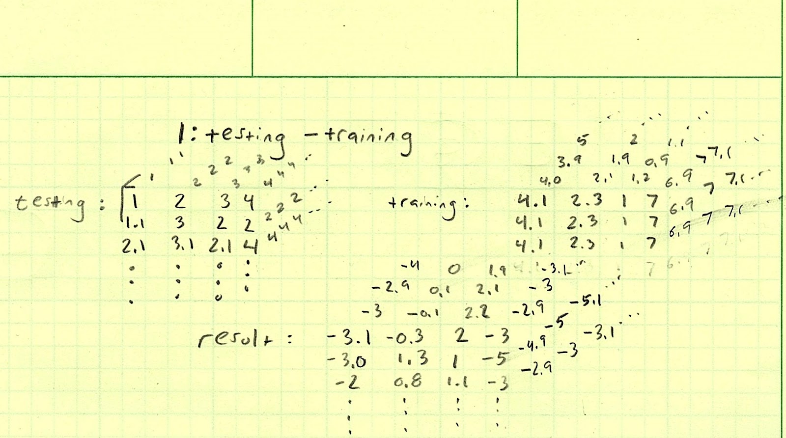
First we do the subtraction, element-wise:
Then we square the result.
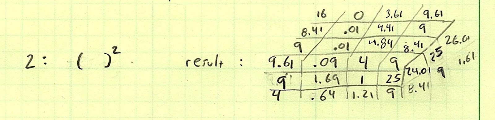
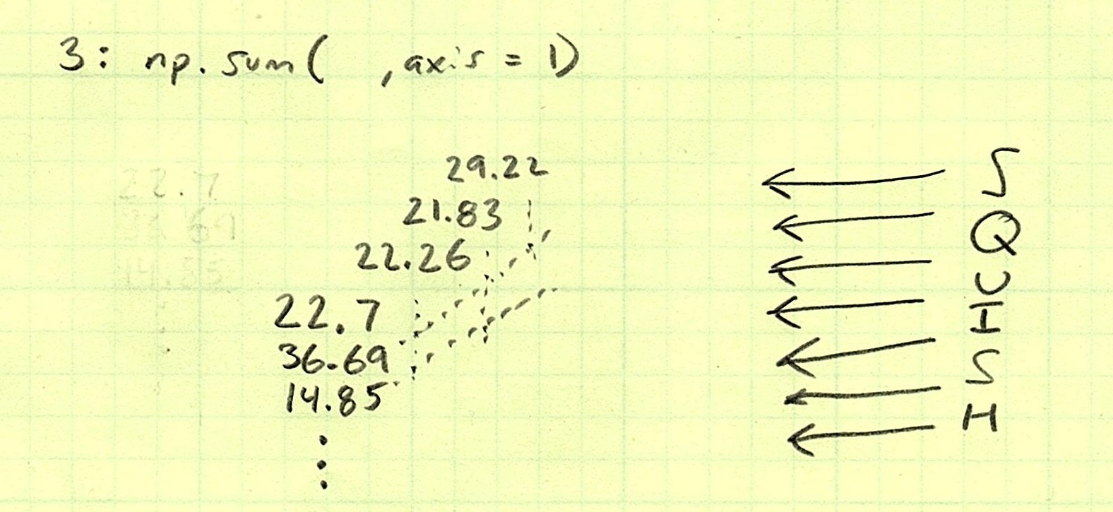
We’re using an aggregating function (sum) to add each column calculation into a single value, which ends up squashing that axis at the end of the day. That’s why we have to tell it which axis to sum across.
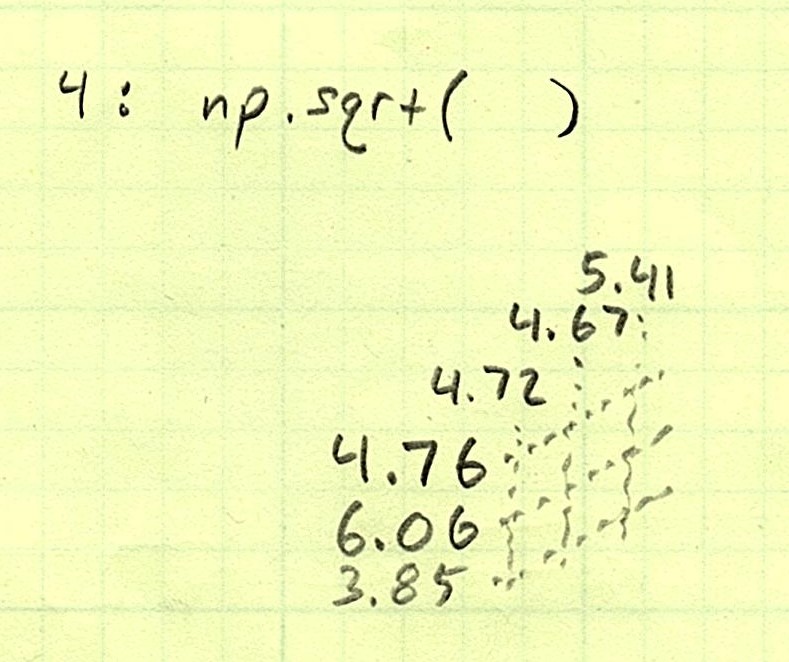
Lastly, take the square root of each number.
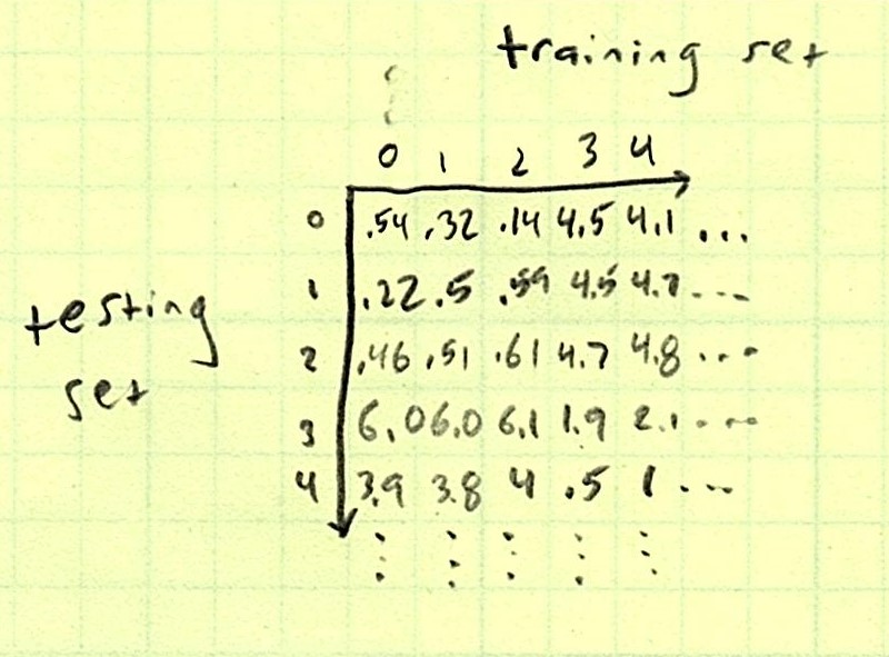
At the end of it all, we’re left with distance array that realistically is 75 x 1 x 75. Conveniently for us, NumPy realizes what we’re going for and swaps the last two axes to get us to a final array of shape 75 x 75. These are the overall 4D distances between each pair of orchids, with testing on the vertical axis and training on the horizontal axis.
It’s all downhill coasting from here on out. If we want to find out which training orchid is closest to each testing orchid, we need to figure out the index of the minimum value for each row.
NumPy provides us with another wonderfully powerful aggregating function argmin that returns the index of the minimum value on a particular axis. Remember again that any time we use an aggregating function, we end up squashing that axis.
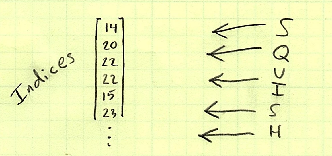
These indices are the indices of the training value that is the most similar to each testing value, element-wise. Let’s see one more piece of vectorized magic: indexing.
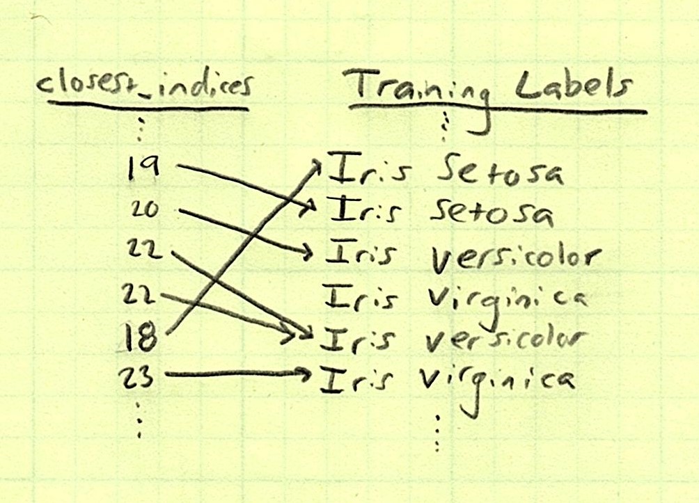
Finally! We have a predicted species of orchid for each test orchid based on the training orchid it was most similar to.
Great work!
Getting Our Data Into Shape
Vectorization and broadcasting are not the easiest concepts to wrap your head around. It’s a pretty thick layer of abstraction that hides a lot of details, but it lifts us programmers up out of the mud and elevates us to allow us to be scientists and mathematicians. If you can master them, you can write the code that you want, the code that you mean, the important code; and you don’t have to obscure it in implementation details like deeply nested loops with intermediate helper variables, clumsy filters, and awkward mapping logic.
Many libraries abstract on top of these array calculations, so you often don’t really have to worry about what shape your data is in throughout the intermediate stages. However, when things go wrong—and they do—understanding multidimensional arrays can really help out.
Now, you’ve got the skills necessary to break those compound vectorized calculations broadcast across differently shaped arrays down. You know how to take each small step of the calculation; figure out what shape the data is in before, during, and after; and determine how that affects the next step of the calculation. This will help keep you from getting overwhelmed and confused and take your data science skills to new heights. Being able to “rotate” data to avoid nested loops and “squash” data with aggregate functions takes your analysis to new dimensions and then brings it back to simpler, more manageable data shapes.
You may not yet have the entire field of data science mastered, but now you are able to properly prepare and shape your data, and these fundamental skills start you off with a solid foundation on which to build your skills.

Related Articles

12 REALITIES of Daily Life as a Programmer
What’s the daily life of a programmer like? A programmer’s daily life consists of auditing and debugging code, coding new…

5G App Development: How To Prepare for the Future of the Internet
5G is the fifth generation of broadband cellular mobile networks and is expected to bring a huge change in the…

Impostor Syndrome as a Programmer
Believing that you’re somewhat unqualified for your job is a problem faced by the best of us. When those thoughts…